Specific arguments for particular field geometry

The openPMD format supports 3 types of geometries:

• Cartesian 2D

• Cartesian 3D

• Cylindrical with azimuthal decomposition (thetaMode)

This notebook shows how to use the arguments of get_field which are specific to a given geometry. You can run this notebook locally by downloading it from this link.

(optional) Preparing this notebook to run it locally

If you choose to run this notebook on your local machine, you will need to download the openPMD data files which will then be visualized. To do so, execute the following cell. (Downloading the data may take a few seconds.)

import os, sys

def download_if_absent( dataset_name ):
    "Function that downloads and decompress a chosen dataset"
    if os.path.exists( dataset_name ) is False:
        import wget, tarfile
        tar_name = "%s.tar.gz" %dataset_name
        url = "https://github.com/openPMD/openPMD-example-datasets/raw/draft/%s" %tar_name
        wget.download(url, tar_name)
        with tarfile.open( tar_name ) as tar_file:
            tar_file.extractall()
        os.remove( tar_name )

download_if_absent( 'example-3d' )
download_if_absent( 'example-thetaMode' )

In addition, we choose here to incorporate the plots inside the notebook.

%matplotlib inline

Preparing the API

Again, we need to import the OpenPMDTimeSeries object:

from openpmd_viewer import OpenPMDTimeSeries

and to create objects that point to the 3D data and the cylindrical data.

(NB: The argument check_all_files below is optional. By default, check_all_files is True, and in this case the code checks that all files in the timeseries are consistent i.e. that they all contain the same fields and particle quantities, with the same metadata. When check_all_files is False, these verifications are skipped, and this allows to create the OpenPMDTimeSeries object faster.)

ts_3d = OpenPMDTimeSeries('./example-3d/hdf5/', check_all_files=False )
ts_circ = OpenPMDTimeSeries('./example-thetaMode/hdf5/', check_all_files=False )

3D Cartesian geometry

For 3D Cartesian geometry, the get_field method has additional arguments, in order to select a 2D slice into the 3D volume: - slice_across allows to choose the axis across which the slice is taken. See the examples below:

# Slice across y (i.e. in a plane parallel to x-z)
Ez1, info_Ez1 = ts_3d.get_field( field='E', coord='z', iteration=500,
                                    slice_across='y', plot=True )

# Slice across z (i.e. in a plane parallel to x-y)
Ez2, info_Ez2 = ts_3d.get_field( field='E', coord='z', iteration=500,
                                    slice_across='z', plot=True )

# Slice across x and y (i.e. along a line parallel to the z axis)
Ez2, info_Ez2 = ts_3d.get_field( field='E', coord='z', iteration=500,
                                    slice_across=['x','y'], plot=True )

• For one given slicing direction, slice_relative_position allows to select which slice to take: slice_relative_position is a number between -1 and 1, where -1 indicates to take the slice at the lower bound of the slicing range (e.g. \(z_{min}\) if slice_across is z) and 1 indicates to take the slice at the upper bound of the slicing range (e.g. \(z_{max}\) if slice_across is z). For example:

# Slice across z, very close to zmin.
Ez2, info_Ez2 = ts_3d.get_field( field='E', coord='z', iteration=500,
     slice_across='z', slice_relative_position=-0.9, plot=True )

When passing slice_across=None, get_field returns a full 3D Cartesian array. This can be useful for further analysis by hand, with numpy (e.g. calculating the total energy in the field).

# Get the full 3D Cartesian array
Ez_3d, info_Ez_3d = ts_3d.get_field( field='E', coord='z', iteration=500, slice_across=None )
print( Ez_3d.ndim )

3

Cylindrical geometry (with azimuthal decomposition)

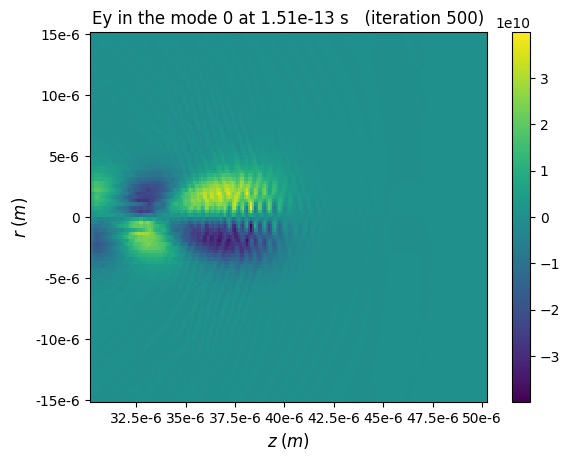
In for data in the thetaMode geometry, the fields are decomposed into azimuthal modes. Thus, the get_field method has an argument m, which allows to select the mode:

• Choosing an integer value for selects a particular mode (for instance, here one can see a laser-wakefield, which is entirely contained in the mode 0)

Ey, info_Ey = ts_circ.get_field( field='E', coord='y', iteration=500, m=0,
                              plot=True, theta=0.5)

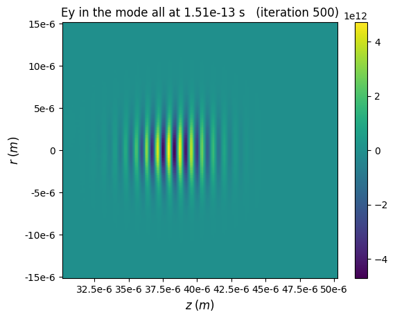
• Choosing m='all' sums all the modes (for instance, here the laser field, which is in the mode 1, dominates the fields)

Ey, info_Ey = ts_circ.get_field( field='E', coord='y', iteration=500, m='all',
                              plot=True, theta=0.5)

The argument theta (in radians) selects the plane of observation: this plane contains the \(z\) axis and has an angle theta with respect to the \(x\) axis.

When passing theta=None, get_field returns a full 3D Cartesian array. This can be useful for further analysis by hand, with numpy (e.g. calculating the total energy in the field), or for comparison with Cartesian simulations.

# Get the full 3D Cartesian array
Ey_3d, info_Ey3d = ts_circ.get_field( field='E', coord='y', iteration=500, theta=None )
print( Ey_3d.ndim )

3

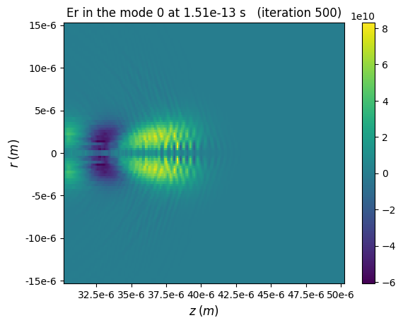
• In cylindrical geometry, the users can also choose the coordinates r and t for the radial and azimuthal components of the fields. For instance:

Er, info_Er = ts_circ.get_field( field='E', coord='r', iteration=500, m=0,
                              plot=True, theta=0.5)

• Finally, in cylindrical geometry, fields can also be sliced, by using the r and z direction. (Keep in mind that slice_across is the direction orthogonal to the slice.)

Er_slice, info = ts_circ.get_field( field='E', coord='r', iteration=500, plot=True, slice_across='r' )

Er_slice, info = ts_circ.get_field( field='E', coord='r', iteration=500, plot=True, slice_across='z' )