Introduction to the openPMD-viewer API

This notebook explains how to use the openPMD-viewer API, in order to access and plot the data stored in a set of openPMD files. You can run this notebook locally by downloading it from this link.

Note that, even though this document is from a Jupyter notebook, the openPMD-viewer API does not require a Jupyter notebook, and can be run in a normal Python environment. It can typically be used to write Python scripts, which perform pre-determined data analysis operations.

(optional) Preparing this notebook to run it locally

If you choose to run this notebook on your local machine, you will need to download the openPMD data files which will then be visualized. To do so, and execute the following cell.

import os

def download_if_absent( dataset_name ):
    "Function that downloads and decompress a chosen dataset"
    if os.path.exists( dataset_name ) is False:
        import wget, tarfile
        tar_name = "%s.tar.gz" %dataset_name
        url = "https://github.com/openPMD/openPMD-example-datasets/raw/draft/%s" %tar_name
        wget.download( url, tar_name )
        with tarfile.open( tar_name ) as tar_file:
            tar_file.extractall()
        os.remove( tar_name )

download_if_absent( 'example-2d' )

In addition, we choose here to incorporate the plots inside the notebook.

%matplotlib inline

Preparing the API

In order to start using the API:

• Load the class OpenPMDTimeSeries from the module openpmd_viewer

from openpmd_viewer import OpenPMDTimeSeries

• Create a time series object by pointing to the folder which contains the corresponding openPMD data

ts = OpenPMDTimeSeries('./example-2d/hdf5/')

Extracting iterations and time values

One can extract all available iterations and corresponding time values from the time series into a numpy array object by doing

it = ts.iterations
time = ts.t

Using the API for the fields

Accessing the field data

The list of available fields is accessible through ts.avail_fields.

The fields can be read with the method get_field.

The user can either require a time (in seconds) or an iteration (an integer). When giving a time, it is not needed to provide the exact time of an available iteration, as the time of the closest available value will be used instead.

# One example
rho, info_rho = ts.get_field( iteration=300, field='rho' )
# Another example
Ex, info_Ex = ts.get_field( t=100.e-15,  field='E', coord='x' )

The method get_field returns two quantities: - A 2D array containing the values of the requested field. - An object containing metainformation about the extent of the grid (e.g info_rho.z and info_rho.x respectively return an array of the z and x positions).

These two objects can then be used in a Python environment to perform numerical analysis.

Plotting the field data

A user could directly plot the extracted array Ex by using e.g. matplotlib’s imshow.

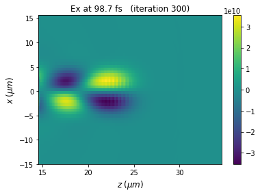
However, for convenience, openPMD-viewer can also directly plot the data, if the argument plot = True is used.

Ex, info_Ex = ts.get_field( t=100.e-15,  field='E', coord='x', plot=True )

Missing or inconsistent argument

If an argument is missing or inconsistent, an exception will be raised and a helper message will be printed.

Additional documentation

Additional documentation on get_field can be obtained by reading its docstring. This can be done for instance by executing the following command in an IPython environment.

ts.get_field?

Moreover, additional documentation about the meta-information object which is returned by get_field can be obtained by adding ? after any metainformation object. For instance:

info_rho?

API for the particles

Accessing the particle data

The particle quantities can be read by using the method get_particle.

Again, the user can give either a physical time, or an iteration. Additionally, the user can request several particle quantities simultaneously, by passing a list of requested quantities (var_list). The method get_particle then returns a list of 1darray (one per requested quantity in var_list, returned in the same order). These 1darrays have one element per macroparticle.

Finally, the user also needs to specify the name of the considered species. The list of available species is accessible through ts.avail_species.

# Look for the available species
print(ts.avail_species)

['Hydrogen1+', 'electrons']

# One example: extracting several quantities
x, y, z = ts.get_particle( var_list=['x','y', 'z'], iteration=300, species='Hydrogen1+')
# Another example: extracting 1 quantity
# (notice the comma after z, so that z is a 1darray, not a list)
z, = ts.get_particle( var_list=['z'], t=150.e-15, species='electrons')

Plotting the particle data

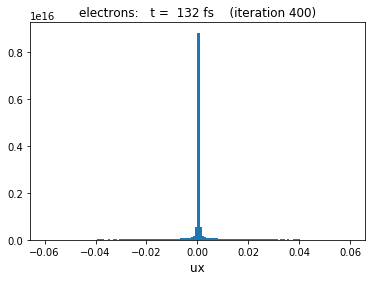
The openPMD-viewer provides plotting support when the argument plot = True is set:

• When only one quantity is requested, a histogram of this quantity is plotted. (This histogram takes into account the weight of the macroparticles.)

ux = ts.get_particle( var_list=['ux'], iteration=400, species='electrons', plot=True )

• When two quantities are requested, a 2d histogram is plotted. (It also takes into account the weight of the macroparticles.)

z, uz = ts.get_particle( var_list=['z','uz'], iteration=400, species='electrons', plot=True, vmax=3e12 )

Missing or inconsistent arguments

As for the fields, if an argument is missing or inconsistent, an exception will be raised and an helper message will be printed.

Additional documentation

As for the get_field method, the documentation on get_particle can be obtained by reading its docstring. This can be done for instance by executing the following command in an IPython environment.

ts.get_particle?

Continue this tutorial

• To learn more about mesh geometries and the corresponding API, look at the notebook 2_Specific-field-geometries.

• To learn about the openPMD-viewer GUI, look at the notebook 3_Introduction-to-the-GUI.